SparSpec software
Sparse modeling for the spectral analysis of unevenly spaced data
New (30th April 2007):
SparSpec version 1.4 is now available
This document in pdf.
SparSpec proposes an alternate approach to estimate frequencies in time series. Indeed, classical sequential methods, that iteratively deconvolve the Fourier spectrum from the effect of the spectral window, can be very sensitive to sampling artifacts and may lead to erroneous results.
The approach used here addresses the problem of fitting multiple sinusoids as the sparse representation of the data in an overcomplete dictionary of pure frequencies. In the signal processing terminology, the latter refers to Basis Pursuit De-Noising while the former sequential approach corresponds to some Matching Pursuit strategy.
Keywords: time series analysis, spectrum estimation, irregular sampling, sparse representations, ℓ1 penalisation.
SparSpec propose une nouvelle approche pour l'estimation de fréquences à partir de séries temporelles. En effet, les méthodes classiques, basées sur la déconvolution itérative du spectre de Fourier, peuvent être très sensibles à la présence d'artéfacts dûs à l'échantillonnage, et peuvent alors déboucher sur des résultats erronés.
L'approche mise en oeuvre ici considère le problème de l'estimation de sinusoides comme la représentation parcimonieuse des données dans un dictionnaire redondant de fréquences pures. Dans le domaine du traitement du signal, cette méthodologie s'inscrit dans les techniques de type Basis Pursuit De-Noising, alors que les approches habituelles séquentielles s'apparentent à des stratégies de type Matching Pursuit.
Mots-clés: analyse de séries temporelles, estimation spectrale, échantillonnage irrégulier, représentations parcimonieuses, pénalisation ℓ1.
Please acknowledge the use of this software in any publication:
"The SparSpec software is available at http://www.ast.obs-mip.fr/Softwares" and cite the reference S. Bourguignon, H. Carfantan and T. Boehm, SparSpec: a new method for fitting multiple sinusoids with irregularly sampled data, Astronomy and Astrophysics, vol. 462, pp. 379-387, Jan 2007 (Preprint here).
Please send a copy of such publication to Herve.Carfantan@irap.omp.eu.
Contents
Let (tn, yn)n=1... N be N samples of available data: the physical quantity yn is obtained at instant tn. Let {xk}k=−P ... P denote the complex-valued amplitude spectrum discretised on a frequency grid of the form {k/Pfmax}k=−P ... P, with arbitrarily small frequency step fmax/P, i.e., arbitrarily large P.
The idea is to find the vector of complex-valued spectral amplitudes that correctly fits the data with the fewest number of non-zero entries: the sparsest spectrum that models the data. A classical approach to do this is to solve the following optimisation problem:
|
= argmin||y − W x||2 + λ Σk |xk|
|
More details about the method can be found in S. Bourguignon et al., SparSpec: a new method for fitting multiple sinusoids with irregularly sampled data, Astronomy and Astrophysics, vol. 462, pp. 379-387, Jan 2007.
Preprint here.
New: SparSpec 1.4 is able to take into account various noise levels in the data. See example of 4.2 for more details.
Important: the SparSpec project is still in its infancy! In particular, depending on your platform, the selected parameters... and on your data, it still may fail, crash or provide inaccurate results.
In this case, please, do not resign! Send your comments and/or bug reports to Herve.Carfantan@irap.omp.eu and we will do our best to help you.
Install the SparSpec package
The SparSpec package gives the sources and executables for Linux (tested with Linux Fedora Core 4 and Ubuntu Dapper) and Windows (tested with Windows XP and Windows 2000).
SparSpec is written in C using GTK+-2.0 for the graphical user interface (GUI).
This program is under the GPL license so you can download the sources and modify them under the terms of this license.
An example of data analysis with SparSpec is given in Section 4.
The Graphical User Interface is divided into four main menus:
-
Data: here you can load the time series you want to analyse, as well as display and plot the corresponding curve. The time series should be a two-column (tn and yn) ascii file MYFILE.dat.
- Parameters: this section allows to select the upper frequency limit fmax and the number of discretised frequencies P (the higher P, the higher the frequency precision... but the longer will be the computation time and the more RAM is required !)
If the data are irregularly sampled, aliasing is pushed at much higher frequencies than for regular sampling and there is no more Nyquist limit. So, select fmax according to some physical knowledge about what you are searching if you can. In this menu, you can plot the spectral window |W(f)| = |Σn e−2iπftn| between −fmax and fmax and the Fourier Spectrum of the data |Y(f)| =|Σn yn e−2iπftn|. Both may help you to select a reasonable value: in particular |W(f)| should be free from any periodicity or pseudo-periodicity (i.e., fmax not too high), but it should also show sidelobes. If not, fmax may not be in adequation with the sampling scheme of your data. The unit of fmax is the inverse of the unit of the instants tn.
- Computation: this is the core of SparSpec. Select a value for parameter λ and start the computation.
Selecting a correct value for λ is still not an automatic issue. However, reasonable bounds can be obtained: if λ is too high, x is identically zero; if λ is too small, then x is not sparse any more.
Parameter λ also has a physical interpretation: for the estimated amplitude spectrum x, λ is the upper bound of the Fourier spectrum of the residual y − W x. See the above referenced paper for more details.
In SparSpec, you enter the normalised value for λ / λmax ∈ [0,1], where λmax = maxk |(W†y)k|. (For λ ≥ λmax one has x=0). In practice, set λ/ λmax to a few percent, e.g., 10%, decrease the value and stop before under-regularisation is reached, that is, when the solution shows many spurious peaks.
After optimisation succeeds, extracted components can be displayed as a table and plotted in the frequency domain, jointly to the initial and residual Fourier spectra. Frequencies are also saved in ascii format in file MYFILE.spec, where MYFILE.dat is the ascii file containing the time series.
- Help: displays a reduced version of this document.
If you do not want to use the GTK-based Graphical User Interface or want to include SparSpec results in an automated procedure, a console mode is also available. To start in console mode, type at the command line:
./SparSpec_nogtk MYFILE.dat
where MYFILE.dat contains the data. This option requires adequate
values for parameters P, fmax and λ / λmax have been stored in configuration file MYFILE.conf. Otherwise, default parameters are used, that may be not optimal. After optimisation succeeds, extracted components are saved in ascii format in file MYFILE.spec.
After the first utilisation with a given time series (stored in a file MYFILE.dat), SparSpec generates a configuration file named MYFILE.conf in ascii format, storing the last set of parameters that were used (fmax, P and normalised λ / λmax). Additional technical parameters are also stored:
-
threshold is a numerical threshold under which complex amplitudes |xk| are considered zero. Its default value is 10−6.
- nitmax is the maximum number of iterations authorised by the optimisation procedure. Its default value is 50000.
- L fixes the frequency the zero values of the iterates are visited in the optimisation procedure. Setting L>1 allows to save up computational time. Its default value is 100.
- relax is a relaxation parameter in the range ]0,2[ used by the Iterative Coordinate Descent procedure, that allows to speed up the optimisation. Its default value is 1.5.
- weight is a binary value parameter which indicates if the various noise levels in the data are taken into account (weight=1) or not (weight=0). See 2.5 for more details and 4.2 for an example.
All these parameters can be modified by editing file MYFILE.conf (see Table 2 for an example of .conf file). Beware: just change the parameter values without modifying the structure of the file.
SparSpec 1.4 is an improved version of SparSpec 1.2.
-
A bug was fixed (when then number of unknown was less than the number of data, SparSpec 1.2 did not converge).
- Initialisation : The optimisation algorithm is initialised with a previous result, if exists. This considerably saves up computational time.
- Graphical display : It is now possible to zoom inside graphical windows using the mouse: zoom in an area by clicking the left button and dragging to draw a rectangle; zoom out with a single left or right click.
- Accounting for various noise levels in the data: a proper noise variance σn2 associated to data yn can be given in the data file as a third column. In such a case, each line of the data file is made of tn, yn and σn2. Such information is taken into account to compute the solution from these weighted data in the least square sense.
If the weighted option is selected, the solution is defined as
|
= argmin
(y − W x)†D2(y − W x) + λ Σk |xk|
|
| Y(f) = |
|
|
|
(yn/σn2) e−2iπ ftn. |
It is still possible to draw the classically defined spectra by selecting the Unweighted option (in Parameters or Computation menus). It is also possible to compute the solution without accounting for the noise variance (select the Unweighted option before computing the solution).
The use of the Unweighted option can also be specified in the .conf file.
See example of 4.2 for more details on estimating frequencies accounting for various noise levels in the data.
Many things have to be done to improve SparSpec, such as:
-
Display a progression bar during computation.
- Display the L-curve to help to choose parameter λ (or any other parameter tuning rule).
- Improve graphical display (print graphs...)
- Monte-Carlo simulations to derive confidence levels on the estimated parameters.
3.1 Bibliography
-
The paper by Gray and Desikachary (1973) may be the first paper on sequential methods to estimate multiple sinusoids: D.F. Gray and K. Desikachary, A new approach to periodogram analyses, The Astrophysical Journal, April 1973, vol. 181, pp. 523–530.
- The cleanest methodology was described by G. Foster (1995). Data in this paper were used in the test example provided in Section 4: G. Foster, The Cleanest Fourier spectrum, The Astronomical Journal, April 1995, vol. 109, pp. 1889–1902.
- The first paper by S.S. Chen et al. (1998) introducing the Basis Pursuit De-Noising:
S.S. Chen, D.L. Donoho and M.A. Saunders, Atomic decomposition by basis pursuit, SIAM Journal on Scientific Computing, 20(1):33–61, 1998.
- The description of SparSpec, applying this methodology to the spectral analysis problem with an own-developed optimisation algorithm:
S. Bourguignon, H. Carfantan and T. Boehm, SparSpec: a new method for fitting multiple sinusoids with irregularly sampled data, Astronomy and Astrophysics, vol. 462, pp. 379-387, Jan 2007.
Preprint here.
-
Period04 is a software implementing a sequential algorithm that also aims at fitting multiple sinusoids. It can be viewed as an implementation of the cleanest strategy, as explained in G. Foster, The Cleanest Fourier spectrum, The Astronomical Journal, 109(4):1889–1902, April 1995.
SparSpec is currently maintained by Hervé CARFANTAN. Many thanks to Ali KHAAZAL and Abdelouahed LASFAR, who contributed to the implementation of this project.
Send any comment, bug report or improvement suggestion at:
Herve.Carfantan@irap.omp.eu
4.1 First example
The artificial data set of our first example is similar to the data proposed by Foster (1995, data set A), which consist in three sinusoids with periods 370, 230 and 100 days and amplitudes 3, 2.828 and 3, respectively. A constant value of 10 is added.
An initial data set was generated with 200 points sampled every 10 days.
The final data sets shows gaps of 100 days every 365 days and gaps of 10 days every 30 days.
To make the problem a bit trickier, a fourth sinusoid was added with period 122.5 days and amplitude 3, such that the sidelobes caused by the annual gaps (for periods 370 and 122.5 day) superimpose at a period of 184 days (1/122.5 - 1/365 = 1/370 + 1/365 = 1/184), generating a high false peak in the Fourier spectrum. White Gaussian noise with standard deviation of 0.3 was also added.
Data are stored in the test.dat file given with the SparSpec package.
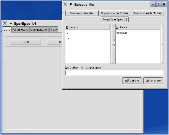
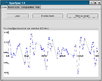
To analyse these data with SparSpec, first call SparSpec and load the data with the load button in the Data menu (see Fig. 1.a). To verify the data are correctly loaded, you can plot them (see Fig. 1.b): the annual gaps can be seen easily.
 |
 |
| a) |
b) |
Figure 1: Load the data and plot the time series.
In the Parameters menu, you now have to set the analysis parameters fmax and P. The mean sampling period of the data is around 13 days so a maximal frequency of 0.5*1/13=3.8 10−2 cycle per day (c/d) is a reasonable first guess.
Note that, for these data, sampling instants were extracted from a regular sampling scheme, so fmax should be set theoretically to less than 0.5* 1/10=5.10−2 c/d to avoid aliasing.
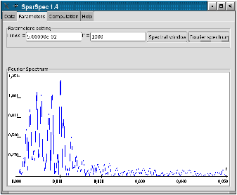
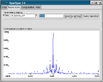
For P=1000, you can verify in the Fourier Spectrum of the data (see Fig. 2.a) that most energy is concentrated under 2.10−2 c/d (for clarity, the mean value of the data was subtracted to plot the spectrum). You can also check the shape of the spectral window (see Fig. 2.b), with its secondary lobes around the frequency 3.10−3 c/d (period 1/365 day).
 |
 |
| a) |
b) |
Figure 2: Fourier Spectrum of the data and spectral window.
In the Computation menu, you have to choose for parameter λ / λmax in [0,1]. Remember that this parameter can be viewed as an upper bound of the Fourier spectrum of the residual, so 10% (relatively to the maximum of the Fourier spectrum of the data) is a realistic first choice. SparSpec results can be displayed as a Table (see Fig. 3.a), a frequency domain plot (see Fig. 3.b) or a time domain plot (see Fig. 3.c). You can verify that SparSpec correctly estimates the four frequencies and amplitudes, as well as the data mean. A fifth frequency is also estimated, but with an amplitude negligible compared to others.
Note that during computation, the shell window displays the state of the optimisation algorithm.
Figure 3: SparSpec results a) list of estimated parameters, b) spectrum of the data and estimated frequencies, c) zoom on the spectrum, d) time representation of the estimated model.
Finally, SparSpec saves results (frequencies, amplitudes and phases) in file test.spec (see table 1) and produces the configuration file test.conf (see table 2) with the parameters used for the computation.
SparSpec results on /tmp/SparSpec/test.dat
for Fmax=0,050000, P=1000 and Lambda/Lambda_max=0,100000

 Frequ.    Ampl.     Phase.
4,773959e-18 9,996442e+00 -1,577745e-11
2,700000e-03 2,974487e+00 1,862453e+00
4,345023e-03 2,808216e+00 -1,570961e+00
5,450000e-03 2,179553e-02 3,772596e-01
8,152573e-03 2,986128e+00 -2,249254e+00
1,000746e-02 2,994560e+00 -1,192582e+00
Table 1: test.spec results file
P = 1000
fmax = 0,050000000000
Lambda/Lambda_max = 0,100000000000
threshold = 1,000000000000e-06
nitmax = 50000
L = 100
relax = 1,500000000000


###################################################################
#                           CAUTION !!!                           #
# This configuration file is generated automatically by SparSpec. #
# You can modify the parameter values.                            #
# Do not modify neither the parameters name nor their order.      #
###################################################################
Table 2: test.conf configuration file
SparSpec 1.4 is able to account for various noise levels in the data: a proper noise variance σn2 associated to data yn can be given in the data file as a third column.
The objective of this second example is to illustrate the use of SparSpec 1.4 in such a case.
4.2.1 Maximum likelihood/least squares amplitude estimation
If the data have the same noise level (supposed additive Gaussian), it is well known that the maximum of the Fourier spectrum corresponds to the maximum likelihood estimation of a single frequency model.
This result can be generalized to various noise levels in the data.
For a given set of frequencies fk, k=−K… K, the amplitude estimation in the least square sense (or in the maximum likelihood sense if noise is considered additive Gaussian) leads to the minimization of criterion
JLS(x) = (y − Wx)†Γ−1(y − Wx),
where W is a Fourier-like matrix: Wn,k = exp(2jπ fk tn) and the noise covariance matrix is diagonal: Γ =E{bb†} = diag{σn2}, with σn2 as nth diagonal element.
Let D = diag{1/σn}, then
JLS(x) = (y − Wx)†D2(y − Wx),
= ||Dy − DWx||2 = ||z − Mx||2,
with weighted data zn = yn/σn and weighted matrix:
Mn,k = 1/σnexp(2jπ fk tn).
For a single frequency fk, the amplitude can be computed as
| xk = (M(fk)†M(fk))−1 M(fk)†z =
|
|
|
|
yn/σn2 e−2jπ fk tn,
|
One can easily show that this weighted Fourier Transform have similar properties than the classical one (linearity, translation, modulation, convolution...)
In particular, if a signal is composed of a sum of complex sinusoids with frequencies fk and amplitudes ak, then the weighted Fourier Transform of this signal is the sum of spectral windows W(f) shifted at frequencies fk with amplitudes ak, where:
4.2.2 Accounting for various noise levels in SparSpec 1.4
In SparSpec 1.4, the noise variance is taken into account: if the weighted option is selected in the Parameters or Computation menus, the solution is defined, as explained above, as
|
= argmin||Dy − DW x||2 + λ Σk |xk|
|
| Y(f) = |
|
|
|
(yn/σn2) e−2iπ ftn. |
4.2.3 An example
The data given in file test_sigma.dat correspond to 3 sinusoids
(of frequencies f1 = 0.1001 c/h (cycle per hour), f2 = 0.12222 c/h and f3 = 0.15555 c/h, off the frequency grid of SparSpec, with respective amplitudes 1, 0.75, and 0.5).
The signal is irregularly sampled to simulate observations during 8 days with two instruments, the first one observing 8 hours every day, the second one observing 8 hours every two days (observing periods between the two instruments are shifted by 8 hours).
Gaussian noise was added to the signal, with fixed variance for each instrument, but the noise variance (σn2) of the first instrument is 100 times larger than that of the second one.
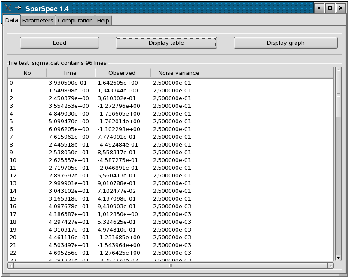
Each line of the data file test_sigma.dat is made of tn, yn and σn2. Data are presented in Fig 4.
 |
 |
| a) |
b) |
Figure 4: Data of file
test_sigma.dat: a) table of values and b) time graph (with error bars at ±σ
n).
It can be seen in Fig. 5 a) and b) that the spectral window, which already has high secondary lobes in the unweighted case due to the periodicity of sampling, is highly modified in the weighted case, for which the secondary lobes are more numerous and of larger amplitude.
Thus, the use of weights highly modify the spectrum of the data as can be seen in Fig. 5 c) and d).
In the unweighted case, the Fourier spectrum shows high peaks at frequencies f1 and f2 and the peak at f3 is totally hidden, due to the sidelobes of the spectral window.
In the weighted case, it is very difficult to analyse the spectrum, although it is statistically more coherent.
Figure 5: Top: spectral windows; bottom: spectrum of the data. Left: unweighted case; right: weighted case.
Frequency estimation with SparSpec, with λ/λmax=30% (the Fourier spectrum of the residual is required to be smaller than 30% of the maximum of the data spectrum), shows similar results in both unweighted and weighted cases, as the three frequencies are correctly estimated, see Fig. 6 a) and b).
However, for λ/λmax=5%, one can see in Fig. 6 c) and d) that the three frequencies are still correctly estimated in the weighted case, while in the unweighted case the number of detected frequencies is much larger than 3.
Figure 6: Spectrum of the data and frequencies estimated with
SparSpec. Top: λ/λ
max = 30%;
bottom: λ/λ
max = 5%.
Left: unweighted case; right: weighted case.
To understand such results, one can compare in Fig. 7 the time representation of the estimated models.
For λ/λmax = 30%, the 3 frequencies are correctly estimated, both in the unweighted and weighted cases.
However, the estimated values ar not strictly identical and
the estimated models have different behaviors.
Indeed, in the weighted case, the model perfectly fits the data with low noise variance, while the distance between the model and the data with larger variance can be greater. In the unweighted case, the whole data are treated the same way, independently of their noise variance.
Thus, one can easily understand that, in order to reduce the residual in the unweighted case (e.g. for λ/λmax = 5%), a greater number of sinusoids is necessary to perfectly fit the model to the data, whatever is their proper noise variance.
This shows the significant improvement that can be reached by accounting for various noise levels in the data.
Figure 7: Time representation of the model estimated with
SparSpec. Top: λ/λ
max = 30%;
bottom: for λ/λ
max = 5%.
Left: unweighted case; right: weighted case.
Finally, SparSpec saves results (frequencies, amplitudes and phases) in file test_sigma.spec (see table 3) and produces the configuration file test_sigma.conf (see table 4) with the parameters used for the computation.
Note that the parameter weight indicates if the computation accounted for the weights in the data (weight=1) or not (weight=0).
SparSpec results on test_sigma.dat with weight=1
for Fmax=0,500000, P=1000 and Lambda/Lambda_max=0,300000

 Frequ.    Ampl.     Phase.
-2,053913e-17 1,159257e-01 -3,141593e+00
1,005000e-01 9,578401e-01 -1,755813e-01
1,215000e-01 7,814625e-01 -2,684308e-01
1,560000e-01 4,837438e-01 1,168614e+00
Table 3: test_sigma.spec results file
P = 1000
fmax = 0,500000000000
Lambda/Lambda_max = 0,300000000000
threshold = 1,000000000000e-06
nitmax = 50000
L = 100
relax = 1,500000000000
weight = 1


###################################################################
#                           CAUTION !!!                           #
# This configuration file is generated automatically by SparSpec. #
# You can modify the parameter values.                            #
# Do not modify neither the parameters name nor their order.      #
###################################################################
Table 4: test_sigma.conf configuration file
This document was translated from LATEX by
HEVEA.